Rotation, SVD, and PCA
DISCLAIMER: This is a blog post from my graduate school years. The blog is no longer maintained and the material might include typos and errors.
Most variables that are of theoretical interest in sociology are not directly observable, i.e., they are latent variables. A problem that plagues every analysis of latent variables is that their scales are arbitrary. Questions such as “what does a unit increas in occupational prestige mean?” or “How much more alienated am I if I am lying two-points higher on the alienation scale than my best friend?” speak to these indeterminacies of latent scales. In order to make sense of such scales, it is often important to “normalize” them. For example, if we have a latent variable $ X $ which has mean $ \mu $ and variance $ \sigma^2 $, we could define a new variable $ Z=(X-\mu)/\sigma $ so that $ E[Z]=0 $ and $ V[Z]=1 $. Now a postive score would imply that I am above average and the magnitude of the score tells us how much, in standard deviation units, I am above the mean, where by standard deviation we mean the standard deviation of the population distribution.
The problem becomes, however, more complicated if $ X $ is multidimensional. Suppose, for example, that we are trying to estimate what Bourdieu called the “social space,” a space of positions defined (very roughly) by two principal axes: the amount and the composition of capital. Say we have come up with some model to do so and are now left with the matrix $ X $ that contains the relative positions in this space. By relative positions, we strees again that the “true” scale of the social space is unobserved or meaningless. Now, what are the columns of $ X $ representing? Ideally, as in Distinction, the y-axis should represent the amount and the x-axis the composition of capital. This might be assured if we have very good items that measure each of the axis such they can be derived from each them separately. Suppose, however, that we do not have this information and, instead, have estimated the space from a survey that asks respondents about their tastes. That is, we have asked respondents how much they like several foods, songs, paintings, etc. In such a situation we can not be sure what the columns of $ X $ represent, even if we have derive somehow a space from it.
It turns out that there is nothing much we can do in these situations. Actually, we do not even know whether the estimated social space is defined in terms of amount and composition of capital: maybe Bourdieu was wrong and it is not the amount and composition of capital but some gene that determines taste; or it might be that each axis represent a different form of capital rather than amount and composition. Thus, we only know that more distant individuals in this space had different patterns of choice with regard to cultural items. What we can do, on the other hand, is to figure out in which directions of this space have the most variation. This would indicate which directions are most important in differentiating between individuals. Then, we might predict the variations by income or education, etc, to see what these directions represent.
But how? The basic idea is to extract from the distribution of positions orthogonal vectors (indicating directions from the origin) and rotate the data points such that the direction that explains most of the variance in the data becomes the first axis, the direction that explains the second most variance the second axis, and so on.
Let us simulate some data, which, say, represent the relative positions in social space.
# load libraries

library('MASS')
library('ggplot2')
library('dplyr')

# generate mean vector and covaraiance matrix

mu <- c(1,-1)
sigma <- matrix(c(1.2,.7,.9,.7),nrow=2)
# check that cov matrix is positive definite

print(eigen(sigma)$value)
[1] 1.7821658 0.1178342
All positive.
# set seed

set.seed(1984)
# generate data

X <- mvrnorm(n=500, mu, sigma)
Let us have a look on the data
# limits for plot

l <- 4
# plot data

ggplot(as.data.frame(X),
       aes(x = V1, y = V2)
    ) +
    labs(x = 'Dim 1', y = 'Dim 2') +
    theme_bw() +
    coord_fixed() +
    geom_vline(xintercept = 0,
               col = 'black',
               linetype = 2) +
    geom_hline(yintercept = 0,
               col = 'black',
               linetype = 2) +
    geom_point(col = 'red3', alpha = .8) +
    lims(x = c(-l, l), y = c(-l, l))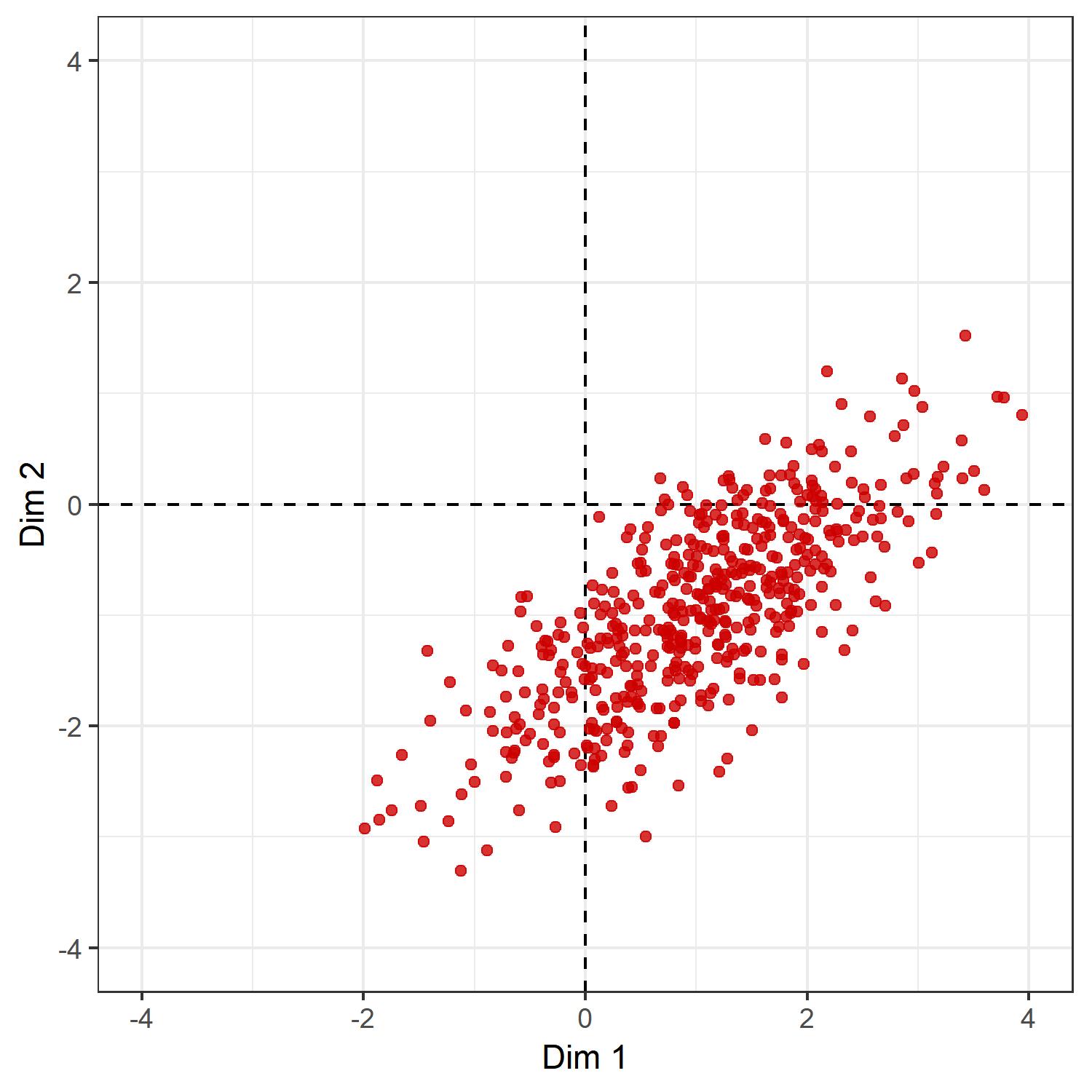
It seems that if we shift the whole distribution a little bit up, then a little bit to the left, and then rotate the positions clockwise by about 45 degrees, we will get the results we want. To do so, we need some basic results from linear algebra.
The first transformtion we are seeking is called “translation.” It is an operation on a coordinate space that moves every point in the same direction by the same amount. Here we want to center the distribution of points at the origin. This can be done by mean-centering each column of the position matrix $ X $. That is, if $ x_1 $ is the first column of $ X $ with mean $ \bar{x}_1 $, then $ z_1 = x_1- \bar{x}_1 $ has a mean $ n^{-1}\sum_j z_1 = n^{-1}\sum_j (x_1 - \bar{x}_1) = 0 $, where $ n $ is the number of rows of $ X $.
# mean-center data

Y <- sweep(X, 2, colMeans(X))
Let $ Y $ be the column-mean centered version of $ Y $, if we plot the points of $ Y $ we get the following:
ggplot(as.data.frame(Y),
       aes(x = V1, y = V2)
    ) +
    labs(x = 'Dim 1', y = 'Dim 2') +
    theme_bw() +
    coord_fixed() +
    geom_vline(xintercept = 0,
               col = 'black',
               linetype = 2) +
    geom_hline(yintercept = 0,
               col = 'black',
               linetype = 2) +
    geom_point(col = 'red3', alpha = .8) +
    lims(x = c(-l, l), y = c(-l, l))
Now, what is left over is the rotation part. Rotation oprations can be done by post-multiplying $ Y $ by a rotation matrix. A rotation matrix, in general, is a sqaure matrix which is 1) orthogonal and 2) has a determinant of 1, i.e., if $ R $ is a rotation matrix, then $ R^{-1}=R^\top $ and $ \text{det}(R)=1 $. The problem is to find the matrix $ R $ that performs the rotation we are seeking: namely a rotation such that the direction of the data with the largest variance becomes our new x-axis. It turns out that this is easier than it seems at first glance.
First, recall that $ Yw $, where $ w $ is a unit vector, will give us the projection of $ Y $ into the direction of $ w $, given that the columns of $ Y $ are centered. As $ Y $ is centered, the $ i $th row of $ Y $, $ y_i $, is a vector from the origin pointing to the $ i $th data point. The cosine of the angle, $ \theta $, between $ y $ an $ w $ is given as $ \cos \theta = \frac{y^\top w}{| y||w| } $. Thus $ | y|\cos \theta $ is the length of the vector $ y $ projected on the line defined by $ w $. But as $ w $ is a unit vector, we have $ | w| =1 $, so that $ \cos \theta | y| =y^\top w $. That is, if $ w $ is defined as the direction of a new axis, $ y^\top w $ gives us the projected length of the vector $ y $ in the direction of that axis.
Now, notice that the sample variance of $ Yw $ is $ n^{-1}(Yw)^\top (Yw) = w^\top (n^{-1}Y^\top Y) w = w^\top S w $. Hence, our problem consists of finding
\[w^*= \text{argmax}_{\{w:\|w\| =1\}} w^\top S w.\]Let $ V $ be a matrix with the eigenvectors of $ S $ stacked in the columns and $ \Lambda $ a matrix with eigenvalues in the diagonals. As $ S $ is symmetric, we can decompose $ S $ into $ S=V\Lambda V^\top $. Substituting this equation into the objective function, we get
\[w^\top S w = w^\top V\Lambda V^\top w = q^\top \Lambda q,\]where $ q= V^\top w $. As $ V $ is orthonormal, we have also that
\[\| q\| = \ V^\top w\| = \sqrt{(V^\top w)^\top (V^\top w)} = \sqrt{w^\top w} = \| w\| =1.\]Thus, the objective function can be rewritten as
\[\sum_{i}\lambda_i q_i^2.\]Let the eigenvalues $ \lambda_i $ of the matrix $ S $ be ordered in decreasing order. Then, it follows immediately that the vector $ q $ that maximizes the sum is $ e_1=[1,0,…,0] $ (as $ q $ has to satisfy $ | q| =1 $, putting only slightest weight to other eigenvalues, which are by definition smaller than $ \lambda_1 $, will decrease the sum). Thus, the vector $ w^* $ we are seeking is given as
\[w^* = V e_1 = v_1,\]i.e., the eigenvector corresponding to the largest eigenvalue of $ S $. Thus, the varaince of the projection will be maximized for the eigenvector corresponding to the largest eigenvalue of $ S $. To find the axis that maximizes the variance of the data in a direction orthogonal to $ v_1 $, we can use the same procedure, except that for the $ i $th direction not only do we need the constraint that $ | w_i| =1 $ but also that $ w_i $ is orthogonal to all $ w_1^{*} , …, w_{i-1}^{*}$. It is not difficult to show that if we proceed in this way, the $ i $th direction will correspond to $ q_i $. The only insight that is needed is that if $ w_2 $ is orthogonal to $ v_1 $, then $ v_1^\top S w_2 = w_2^\top S v_1 = w_2^\top \lambda v_1 = \lambda w_2^\top v_1 = 0 $, i.e., $ S w_2 $ is also orthogonal to $ v_1 $.
Therefore, the rotation we want is given by the matrix $ V $ which contains the eigenvectors of $ S $. Indeed,by definition $ V^{-1}=V^\top $ and $ \text{det}(I) = \text{det}(V^\top V) = \text{det}(V^\top)\text{det}(V)=1 $, so that it follows that $ \text{det}(V)=1 $ or $ -1 $ (where $ \text{det}(V)=-1 $ would imply that the rotation induced by $ V $ includes also a reflection around the origin). Hence, $ V $ satisfies the conditions of a rotation matrix. To obtain this matrix, we can use the singular value decomposition of $ Y=U\Sigma V^\top $. The matrix of right-singular vectors will be equal to the matrix of eigenvectors of $ S $ and hence $ V $.
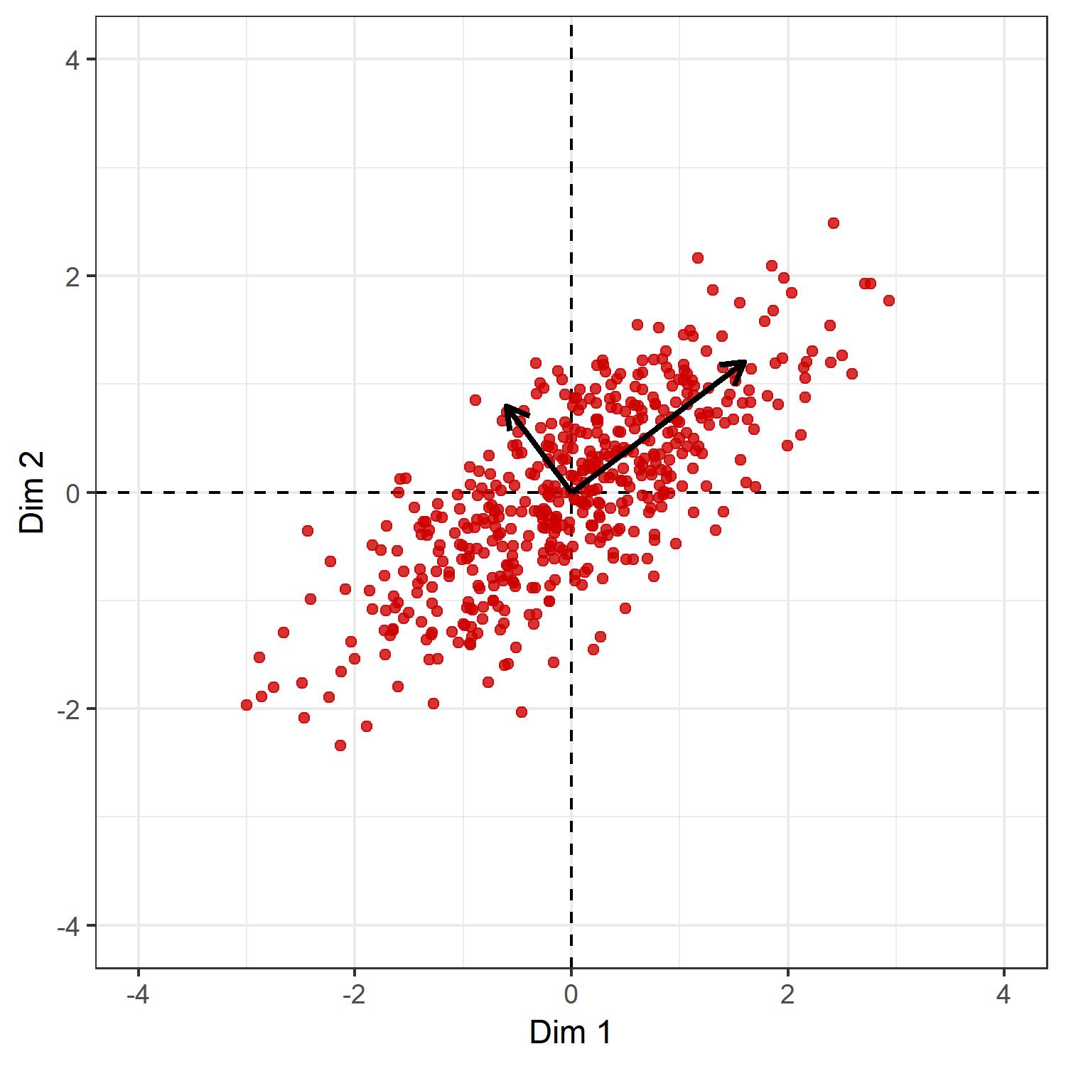
Let us have a look at the direction of the columns of $ V $.
# SVD

SVD <- svd(Y)
# singular values

s.val <- SVD$d
# right singular vectors

v.vecs <- SVD$v
# left singular vectors

u.vecs <- SVD$u
# if determinant is -1 reflect around first vector

if(det(v.vecs) == -1)
    v.vecs <- v.vecs %*% diag(c(1,-1))

# scale right singular vectors by singular values

ggplot(as.data.frame(Y),
       aes(x = V1, y = V2)
    ) +
    labs(x = 'Dim 1', y = 'Dim 2') +
    theme_bw() +
    coord_fixed() +
    geom_vline(xintercept = 0,
               col = 'black',
               linetype = 2) +
    geom_hline(yintercept = 0,
               col = 'black',
               linetype = 2) +
    geom_point(col = 'red3', alpha = .8) +
    lims(x = c(-l, l), y = c(-l, l)) +
    geom_segment(
        data = as.data.frame(
            t(v.vecs %*% diag(c(2,1)))
        ),
        aes(x = 0, y = 0,
            xend = V1, yend = V2
        ),
        size = 1,
        arrow = arrow(
            length = unit(.3, 'cm')
        )
    )
Now, the matrix $ Z=YV $ will contain the rotated positions we are seeking. To see why, let $ y_i^\top $ be any row of $ Y $. Then $ z_i=y_i^\top V $ is the rotation operation $ V $ applied to this row. Now, the rotation matrix for two-dimensional Euclidean spaces is usually formulated as:
\[R_\theta =\begin{bmatrix} \cos \theta & -\sin \theta \\ \sin\theta & \cos\theta\end{bmatrix}.\]The angle of rotation that the matrix $ V $ induces is thus
# in radians

acos(v.vecs[1,1])
[1] 0.6462543
# in degrees

180*acos(v.vecs[1,1])/pi
[1] 37.02764
roughly what is expected from the picture. Hence, each row of $ Y $ is rotated into the coordinate system defined by $ (v_1,v_2) $, with $ v_1 $ being in the direction of maximal variance and $ v_2 $ being orthogonal to it.
Let me elaborate a little bit on this point, since we were talking about rotation and projection quite interchangably and the relationship between these two might not be clear at first glance. The relationship might be explained as follows: consider an arbitrary point in the current coordinate system that has, say, $ y^\top =(1, 2) $. To make the example concrete, let us plot it.
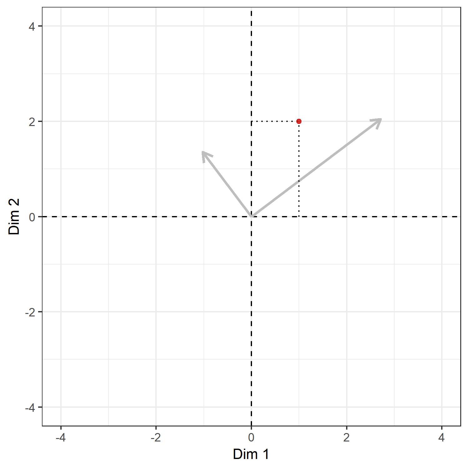
The grey arrows show the directions of the right-singular vectors and the dotted lines the coordinates in the current system, namely the $xy$-plane. As discussed above, post-multiplying this vector, namely $ (1,2) $, by the right-singular vectors $ V=[v_1,v_2] $ will give us the projection in the direction of $ v_1 $ and $ v_2 $. This looks something like:

Again, the dotted lines show the coordinates of the point in the system defined by the right-singular vectors. But these vectors are the new axes we want! Hence, if we treat the two singular vectors as our $x$- and $y$-axis, the picture would look something like this:
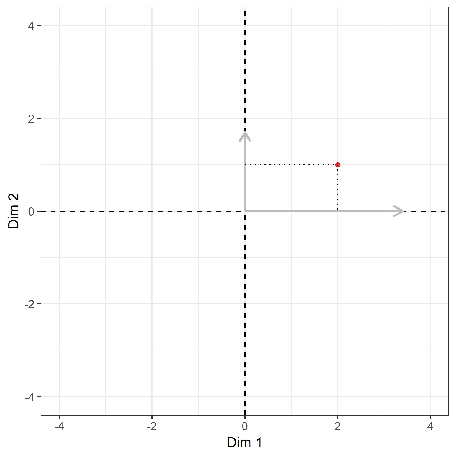
Thus, the whole operation of rotation can also be understood as a change-of-basis operation. This makes intuitive sense: we might hold the position of the points constant and rotate the coordinate system (change of basis), or we keep the coordinate system constant and rotate the points (rotation); regardless of how we perceive the process, the result will be the same.
Now, let us plot $ Z $, where we add the original distribution of the points $ X $ in gray:
# get rotated positions

Z <- Y %*% v.vecs

# plot

ggplot(as.data.frame(Z),
       aes(x = V1, y = V2)) +
    labs(x = 'Dim 1', y = 'Dim 2') +
    geom_point(
        data = as.data.frame(X),
        col = 'grey', alpha = .3) +
    theme_bw() +
    coord_fixed() +
    geom_vline(
        xintercept = 0,
        col = 'black',
        linetype = 2
    ) +
    geom_hline(
        yintercept = 0,
        col = 'black',
        linetype = 2
    ) +
    geom_point(col = 'red3', alpha = .8) +
    lims(x = c(-l, l), y = c(-l, l))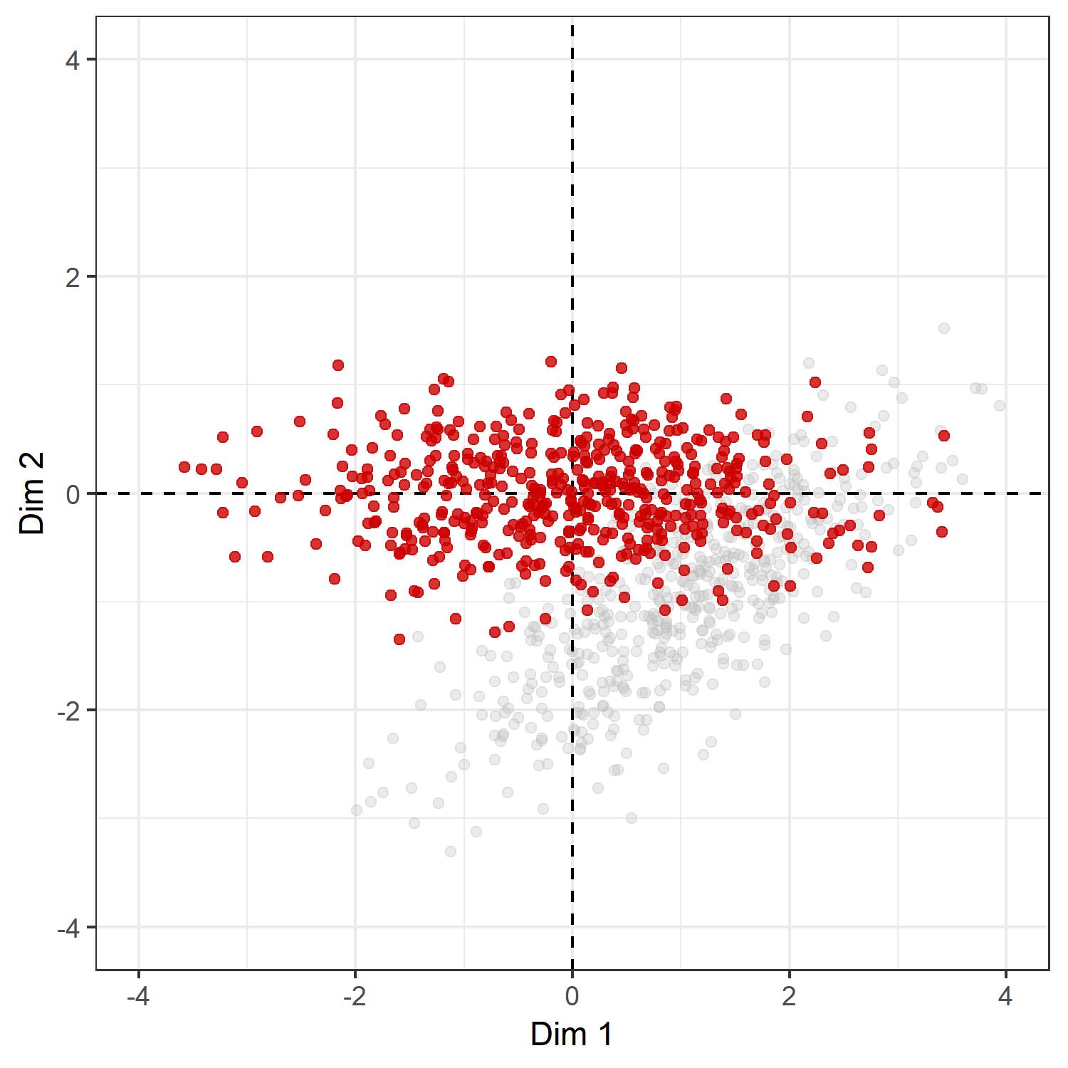
Voila :) As the operation is a rotation, the distances between the points in $ X $ and $ Z $ are all equal. We have simply translated the points, so that the center of the point cloud lies at the origin, and then have rotated the points, such that the x-axis gives the direction of maximal variation. We can also check whether this is indeed true:
# distance matrix, X

d.X <- dist(X) %>% as.matrix
# distance matrix, Z

d.Z <- dist(Z) %>% as.matrix
# sum of squared differences

sum((d.X-d.Z)^2)
[1] 1.235519e-26
Virtually zero. Now, we might use the first and second dimension as our outcome to look at which predictors explain variation across these directions, in the hope that occupation and education have high predictive power.
Yet, there is also another important thing that we can do with the singular value decomposition. Say, we want a unidimensional index of the social space. Ignoring Bourdieu’s scronful view of these indices, which are according to him, par excellence, the destroyers of structures, let us think of best way to do so. As we have seen above, the first right-singular vector gives us the direction that maximizes the variation of data points. It turns out that if we would use only the first left-singular vector, singular value, and right-singular vector of the singular value decomposition to generate $ \tilde Y = u_1 \sigma_1 v_1^\top $, the resulting matrix $ \tilde Y $ will be the best approximation to the original matrix $ Y $ in the sense that it minimizes the norm $ | Y-\tilde Y| $, where the norm $ | \cdot| $ is either the spectral norm or the Forbenious norm. This result is known as the Eckart-Young Theorem. In statistics, the solution so obtained is sometimes called the total least-squares solution, which can be understood as the line which minimizes the squared perpendicular distance from each data point to the reduced space (here, it will be a line). Note that this solution will be different from the ordinary least-squares solution, where the squared vertical distance is minimized.
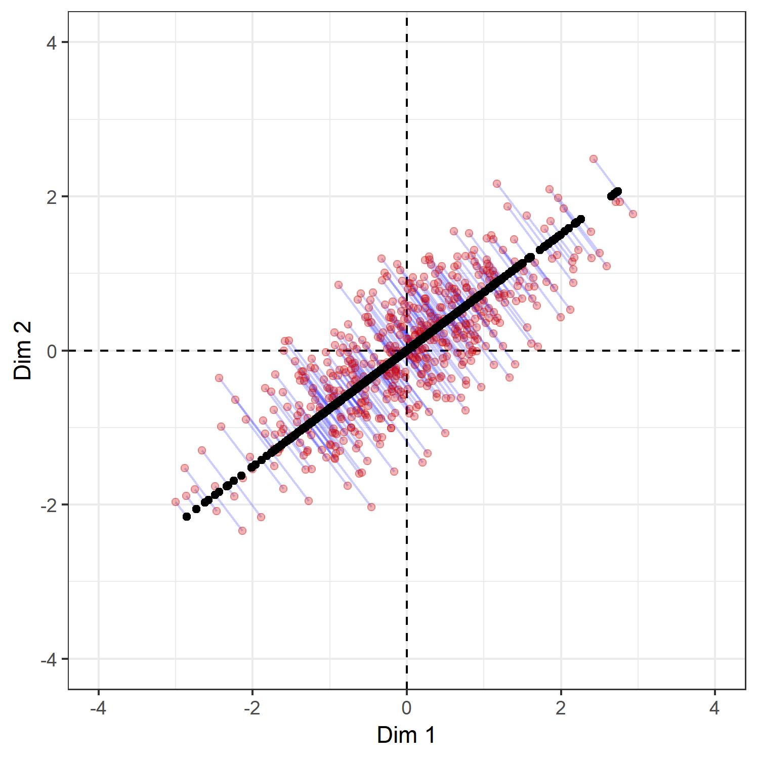
For example, the following plot shows the line created by a rank-one approximation to $ Y $, where the original points of $ Y $ are shown in red, the new points $ \tilde Y $ in black, and where the light blue lines show where each point in $ Y $ is mapped to in $ \tilde Y $. It turns out that for no other line will be the squared length of the blue lines be smaller than the current one.
# rank-one approximation to original matrix

tilde.Y <- s.val[1] * u.vecs[, 1] %*% t(v.vecs[, 1])

# mapping from original matrix to approximation

mapping.tilde.Y <- cbind(Y, tilde.Y)

# plot

ggplot(
    as.data.frame(tilde.Y),
    aes(x = V1, y = V2)) +
    labs(x = 'Dim 1', y = 'Dim 2') +
    geom_vline(
        xintercept = 0,
        col = 'black',
        linetype = 2
    ) +
    geom_hline(
        yintercept = 0,
        col = 'black',
        linetype = 2
    ) +
    theme_bw() +
    coord_fixed() +
    geom_segment(
        data = as.data.frame(mapping.tilde.Y),
        aes(x = V1, y = V2, xend = V3, yend = V4),
        col = 'blue', alpha = .2) +
    geom_point(mapping = aes(x = V1, y = V2),
        data = as.data.frame(Y),
        col = 'red3', alpha = .3) +
    geom_point(col = 'black') +
    lims(x = c(-l, l), y = c(-l, l))